Exploring Echoregions Lines Functionality#
This notebook parses seafloor values from an Echoview .evl file and creates a seafloor mask for the corresponding Echogram data.
# Importing Packages
import matplotlib.pyplot as plt
import urllib.request
import shutil
import xarray as xr
import numpy as np
import pandas as pd
from pandas.testing import assert_frame_equal

import echoregions as er
seafloor Data Reading#
To start this tutorial, we first download evl data from Echoregions’ Github Repository and parse the .evl file using Echoregions’ read_evl function.
The parsing is based off of the .evl data description shown on Echoview’s website: Line Attributes.
# Set path to notebook data
NOTEBOOK_DATA_PATH = 'https://raw.githubusercontent.com/OSOceanAcoustics/echoregions/store_notebook_data/docs/source/notebook_data'

# Download example EVL File
urllib.request.urlretrieve(f"{NOTEBOOK_DATA_PATH}/transect_notebook.evl","transect_notebook.evl")

# Read EVL file
lines = er.read_evl('transect_notebook.evl')
Lines as a DataFrame#
lines is a specialized object but it has a data attribute which is a simple dataframe.
# Grab lines dataframe
lines_df = lines.data
lines_df
| file_name | file_type | evl_file_format_version | echoview_version | time | depth | status | |
|---|---|---|---|---|---|---|---|
| 0 | transect_notebook.evl | EVBD | 3 | 13.0.378.44817 | 2019-07-02 16:00:24.619000 | 95.547655 | 3 |
| 1 | transect_notebook.evl | EVBD | 3 | 13.0.378.44817 | 2019-07-02 16:00:25.114300 | 95.550143 | 3 |
| 2 | transect_notebook.evl | EVBD | 3 | 13.0.378.44817 | 2019-07-02 16:00:25.115300 | 95.701600 | 3 |
| 3 | transect_notebook.evl | EVBD | 3 | 13.0.378.44817 | 2019-07-02 16:00:28.093000 | 94.650797 | 3 |
| 4 | transect_notebook.evl | EVBD | 3 | 13.0.378.44817 | 2019-07-02 16:00:47.767300 | 93.716749 | 3 |
| ... | ... | ... | ... | ... | ... | ... | ... |
| 6042 | transect_notebook.evl | EVBD | 3 | 13.0.378.44817 | 2019-07-02 20:17:16.086000 | 374.501271 | 3 |
| 6043 | transect_notebook.evl | EVBD | 3 | 13.0.378.44817 | 2019-07-02 20:17:17.457000 | 374.999600 | 3 |
| 6044 | transect_notebook.evl | EVBD | 3 | 13.0.378.44817 | 2019-07-02 20:17:18.817000 | 376.674986 | 3 |
| 6045 | transect_notebook.evl | EVBD | 3 | 13.0.378.44817 | 2019-07-02 20:17:20.188000 | 375.435050 | 3 |
| 6046 | transect_notebook.evl | EVBD | 3 | 13.0.378.44817 | 2019-07-02 20:17:21.567000 | 377.058786 | 3 |
6047 rows × 7 columns
Note the rightmost column status. Status values are generally described by the following:
0 = none
1 = unverified
2 = bad
3 = good
The good and bad values are assigned via the specific EVL line picking formula used to generate the initial EVL file. Generally, we only want the rows with good/3 status.
More information on Line Status can be found here: Line Status.
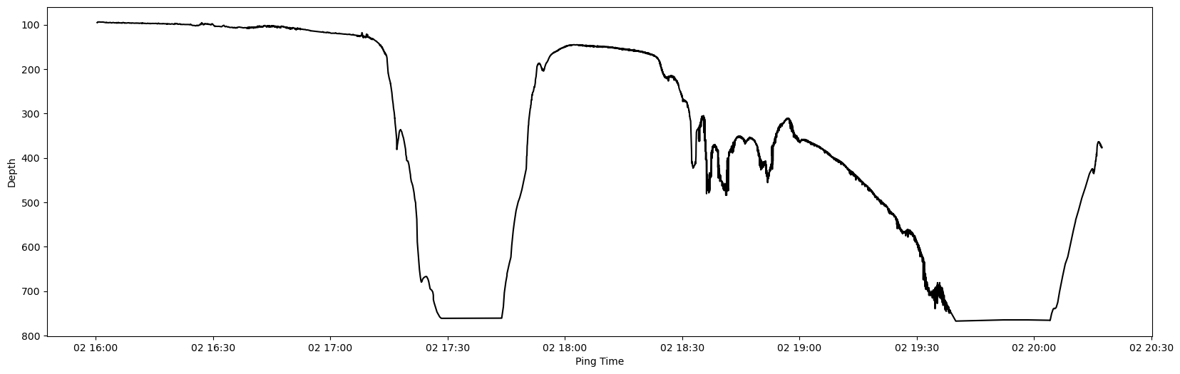
Let’s now plot good points.
# Status 3 are good points so we select those
good_lines_df = lines_df[lines_df['status'] == '3']
good_seafloor = good_lines_df[['time', 'depth']]

plt.figure(figsize=(20, 6))
plt.plot(good_seafloor['time'], good_seafloor['depth'], c='black')
plt.xlabel('Ping Time')
plt.ylabel('Depth')
plt.gca().invert_yaxis()

plt.show()
For usage later on, set this good dataframe as the current line dataframe:
lines.data = good_lines_df
Echogram Data Reading and Plotting#
Let’s now download a zip file containing backscatter data and plot an echogram created using Echopype. Echopype is a comprehensive software designed for parsing sonar backscatter and conducting scientific computations. It offers a wide array of functionalities, including the plotting of echograms, which are visual representations formed by the echoes received from sonar signals. Additionally, Echopype seamlessly integrates with Echoregions, a specialized software for parsing echogram annotations. For now, we will primarily be working with the ds_Sv["Sv"] backscatter volume data variable, which when plotted becomes an echogram, but there are many more data variables that can be used when working with Echopype.
# Download example Echopype Sv Zarr File
urllib.request.urlretrieve(f"{NOTEBOOK_DATA_PATH}/transect_notebook.zip","transect_notebook.zip")

# Extract the ZIP file
shutil.unpack_archive("transect_notebook.zip", "../../")

# Read subset of volume backscattering strength (Sv) data
ds_Sv = xr.open_dataset('transect_notebook.zarr', engine="zarr").sel(
    ping_time=slice("2019-07-02T16:00:00", "2019-07-02T20:10:00")
)
ds_Sv["Sv"]
<xarray.DataArray 'Sv' (channel: 2, ping_time: 3001, depth: 380)> Size: 18MB
[2280760 values with dtype=float64]
Coordinates:
* channel (channel) <U37 296B 'GPT 18 kHz 009072058c8d 1-1 ES18-11' 'GP...
* ping_time (ping_time) datetime64[ns] 24kB 2019-07-02T16:00:00 ... 2019-0...
* depth (depth) float64 3kB 0.0 2.0 4.0 6.0 ... 752.0 754.0 756.0 758.0
Attributes:
binning_mode: physical units
cell_methods: ping_time: mean (interval: 5 second comment: ping_...
long_name: Mean volume backscattering strength (MVBS, mean Sv...
ping_time_interval: 5s
range_meter_interval: 2.0m
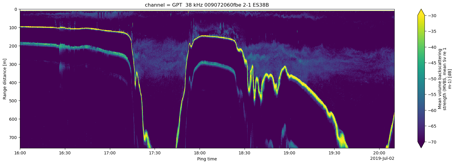
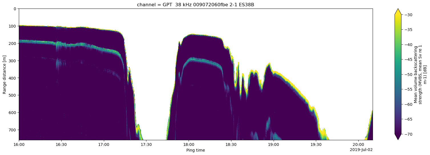
units: dB# Plot the 38 kHz backscatter channel
plt.figure(figsize = (20, 6))
ds_Sv["Sv"].isel(channel=1).plot.pcolormesh(y="depth", yincrease=False, vmin=-70, vmax=-30)
<matplotlib.collections.QuadMesh at 0x7d0f83521f10>
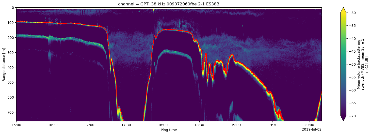
Plotting Echogram and seafloor#
From the two previous plots, we can see how they’re related on both the depth and time dimensions. Now let’s see seafloor annotations overlayed on top of the Echogram dataset.
# Plotting the Echogram data and the seafloor
plt.figure(figsize = (20, 6))
plt.plot(lines.data['time'], lines.data['depth'], 'red', fillstyle='full', markersize=1)
ds_Sv.Sv.isel(channel=1).T.plot.pcolormesh(y="depth", yincrease=False, vmin=-70, vmax=-30)
<matplotlib.collections.QuadMesh at 0x7d0f82f0e600>
Creating Echogram Mask with seafloor#
We can see that there is clear overlap between the two pieces of data here. However, for machine learning training purposes, or for biomass estimation, it is necessary to mask out the pixels below the seafloor line.
The Lines class has a function to do this specific task: mask. The mask function interpolates the seafloor points found in the DataFrame to generate new seafloor points, and from these new points, generates an Xarray seafloor mask. There are a few different Pandas interpolation schemes we can pass in, but for this example we stick with something simple slinear which refers to a first order spline.
# Use the built in mask function
seafloor_mask_da, seafloor_points = lines.seafloor_mask(
    ds_Sv["Sv"].isel(channel=1).drop_vars("channel").compute(),
    operation="above_below",
    method="slinear",
    limit_area=None,
    limit_direction="both"
)
/home/exouser/miniforge3/envs/echoregions/lib/python3.12/site-packages/pandas/core/indexes/base.py:7654: FutureWarning: Dtype inference on a pandas object (Series, Index, ExtensionArray) is deprecated. The Index constructor will keep the original dtype in the future. Call `infer_objects` on the result to get the old behavior.
  return Index(sequences[0], name=names)
Note that selecting 1 channel here is to ensure that our output is a single channel mask. The number of channels of the data array that is passed into the mask will match the number of channels of the output seafloor mask data array.
The output should be both the seafloor mask itself (seafloor_mask_da) and interpolated points that constitute the seafloor mask (seafloor_points).
Let’s take a look at the mask seafloor_mask_da first:
seafloor_mask_da
<xarray.DataArray (depth: 380, ping_time: 3001)> Size: 9MB
array([[0, 0, 0, ..., 0, 0, 0],
       [0, 0, 0, ..., 0, 0, 0],
       [0, 0, 0, ..., 0, 0, 0],
       ...,
       [1, 1, 1, ..., 1, 1, 1],
       [1, 1, 1, ..., 1, 1, 1],
       [1, 1, 1, ..., 1, 1, 1]], shape=(380, 3001))
Coordinates:
  * depth      (depth) float64 3kB 0.0 2.0 4.0 6.0 ... 752.0 754.0 756.0 758.0
  * ping_time  (ping_time) datetime64[ns] 24kB 2019-07-02T16:00:00 ... 2019-0...
Attributes:
    binning_mode:          physical units
    cell_methods:          ping_time: mean (interval: 5 second comment: ping_...
    ping_time_interval:    5s
range_meter_interval: 2.0mThe values in the seafloor mask should also just be 1s (at and below seafloor) and 0s (above seafloor):
print("Unique Values in seafloor Mask:", np.unique(seafloor_mask_da.data))
Unique Values in seafloor Mask: [0 1]
As a sanity check, let us check that the ping_time and depth dimensions in the seafloor mask seafloor_mask_da are equal to that in the backscatter data ds_Sv["Sv"]:
print("seafloor Mask Ping Time Dimension Length:", len(seafloor_mask_da["ping_time"]))
print("seafloor Mask Depth Dimension Length:", len(seafloor_mask_da["depth"]))
print("Echogram Ping Time Dimension Length:", len(ds_Sv["Sv"]["ping_time"]))
print("Echogram Depth Dimension Length:", len(ds_Sv["Sv"]["depth"]))
seafloor Mask Ping Time Dimension Length: 3001
seafloor Mask Depth Dimension Length: 380
Echogram Ping Time Dimension Length: 3001
Echogram Depth Dimension Length: 380
A plot of the mask itself:
plt.figure(figsize = (20, 6))
seafloor_mask_da.plot(y="depth", yincrease=False)
<matplotlib.collections.QuadMesh at 0x7d0f80159910>
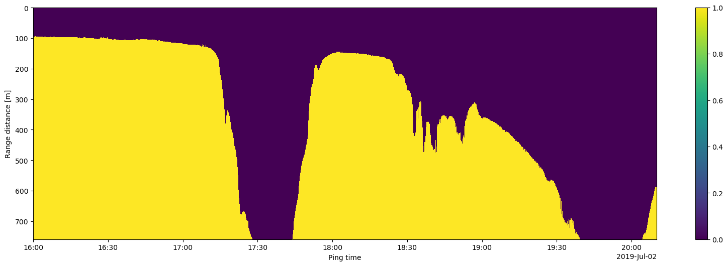
A plot of the 38 kHz channel where the mask is 1:
# Get only 38 kHz channel values where the mask is 1
mask_exists_Sv = xr.where(
    seafloor_mask_da == 1,
    ds_Sv["Sv"].isel(channel=1),
    np.nan,
)

# Plot the masked Sv
plt.figure(figsize = (20, 6))
mask_exists_Sv.plot.pcolormesh(y="depth", yincrease=False, vmin=-70, vmax=-30)
<matplotlib.collections.QuadMesh at 0x7d0f78580290>
Let’s now take a look at the interpolated points seafloor_points:
Let’s compare its number of rows to the number of rows from the lines dataframe it was created from.
print("Interpolated Rows:", len(seafloor_points))
print("Original Rows:", len(lines.data))
Interpolated Rows: 3001
Original Rows: 5361
Why are there more rows in the original rows than there are in the intepolated rows? It’s because the interpolated seafloor data has to match the ping time dimension of the passed in dataset.
Let’s now look at the Echogram ping time dimension length:
print("Echogram Ping Time Dimension Length:", len(ds_Sv["ping_time"]))
Echogram Ping Time Dimension Length: 3001
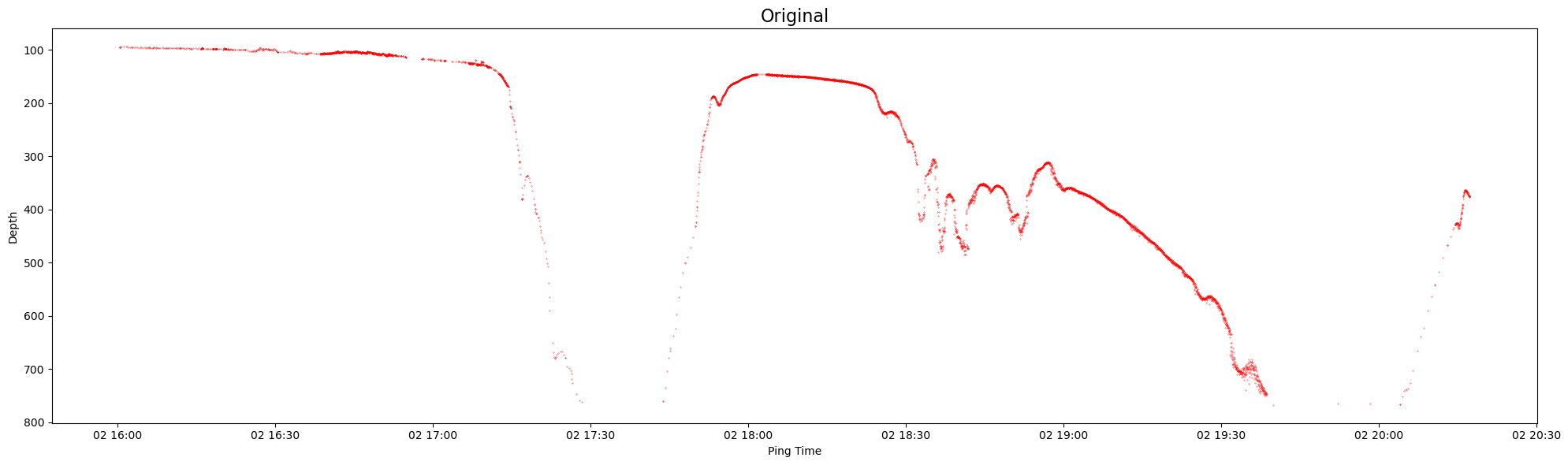
Let’s now plot original seafloor points vs interpolated points:
# Plot both original and interpolated
plt.figure(figsize = (20, 6))
plt.plot(lines.data['time'], lines.data['depth'], 'r.', markersize=0.5)
plt.gca().invert_yaxis()
plt.title('Original', fontsize=16)
plt.xlabel('Ping Time')
plt.ylabel('Depth')
plt.tight_layout()
plt.show()
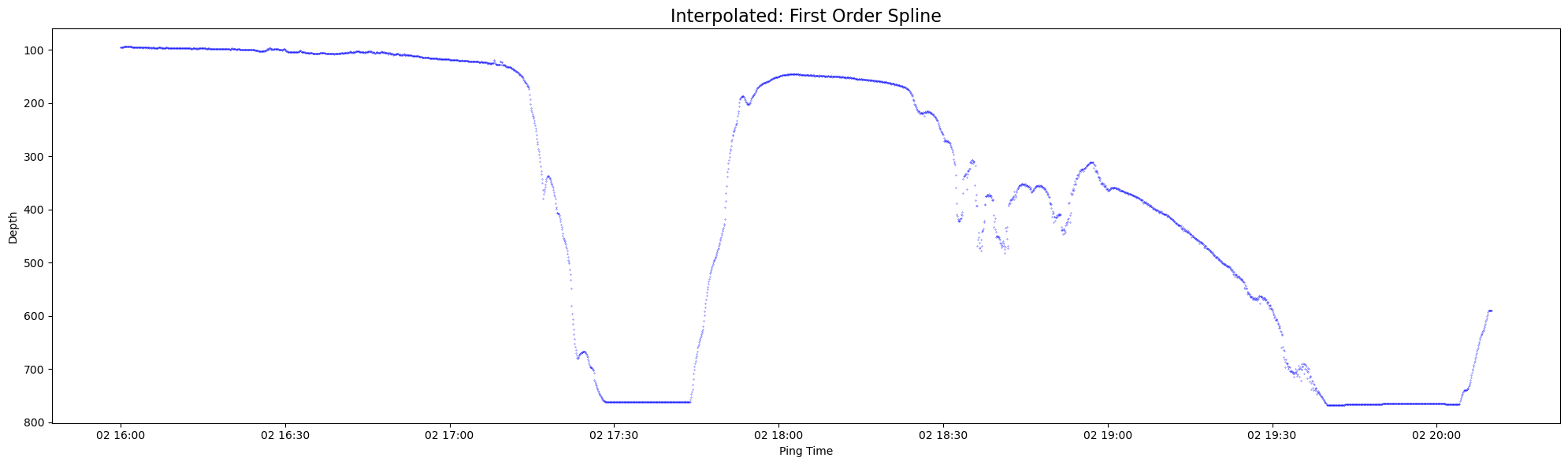
plt.figure(figsize = (20, 6))
plt.plot(seafloor_points['time'], seafloor_points['depth'], 'b.', markersize=0.5)
plt.gca().invert_yaxis()
plt.title('Interpolated: First Order Spline', fontsize=16)
plt.xlabel('Ping Time')
plt.ylabel('Depth')
plt.tight_layout()
plt.show()
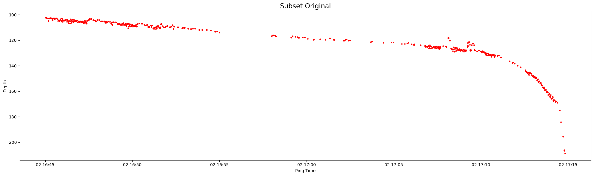
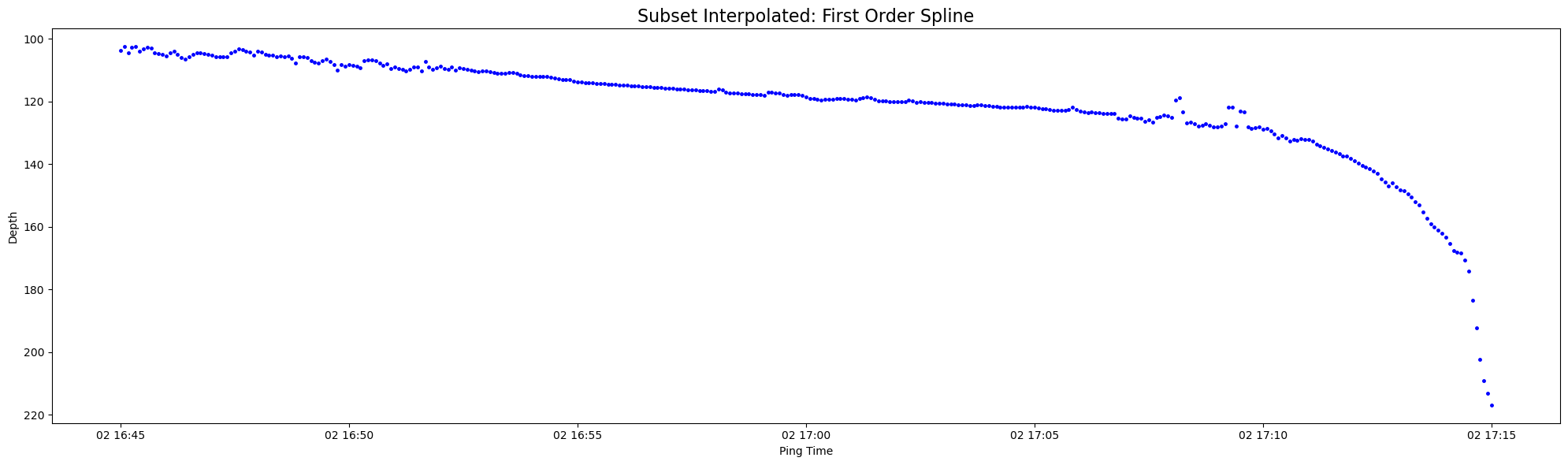
Let’s now look at a 30 minute subset of original and interpolated data between 2019-07-02 16:45:00 and 2019-07-02 17:15:00:
# Filter the DataFrames based on time range
start_time = pd.to_datetime('2019-07-02 16:45:00')
end_time = pd.to_datetime('2019-07-02 17:15:00')
subset_lines_data = lines.data[(lines.data['time'] >= start_time) & (lines.data['time'] <= end_time)]
subset_seafloor_points = seafloor_points[(seafloor_points['time'] >= start_time) & (seafloor_points['time'] <= end_time)]

# Plot both original and interpolated
plt.figure(figsize = (20, 6))
plt.plot(subset_lines_data['time'], subset_lines_data['depth'], 'r.', markersize=5)
plt.gca().invert_yaxis()
plt.title('Subset Original', fontsize=16)
plt.xlabel('Ping Time')
plt.ylabel('Depth')
plt.tight_layout()
plt.show()

plt.figure(figsize = (20, 6))
plt.plot(subset_seafloor_points['time'], subset_seafloor_points['depth'], 'b.', markersize=5)
plt.gca().invert_yaxis()
plt.title('Subset Interpolated: First Order Spline', fontsize=16)
plt.xlabel('Ping Time')
plt.ylabel('Depth')
plt.tight_layout()
plt.show()
Note that ds_Sv is the entire dataset containing many data variables that Echoregions does not work with, and so passing in the entire dataset to Echoregions lines.mask will produce an error since it expects a single data array ds_Sv["Sv"]:
# Test ds_Sv
lines.seafloor_mask(
    ds_Sv,
    method="slinear",
    limit_area=None,
    limit_direction="both"
)
---------------------------------------------------------------------------
TypeError                                 Traceback (most recent call last)
Cell In[24], line 2
      1 # Test ds_Sv
----> 2 lines.seafloor_mask(
      3     ds_Sv,
      4     method="slinear",
      5     limit_area=None,

File ~/echoregions/echoregions/lines/lines.py:278, in Lines.seafloor_mask(self, da_Sv, operation, **kwargs)
    219 """
    220 Subsets a seafloor dataset to the range of an Sv dataset. Create a mask of
    221 the same shape as data found in the Echogram object:
   (...)    274     from each other.
    275 """
    277 if not isinstance(da_Sv, DataArray):
--> 278     raise TypeError(
    279         f"Input da_Sv must be of type DataArray. da_Sv was instead of type {type(da_Sv)}"
    280     )
    282 if operation not in ["regionmask", "above_below"]:
    283     raise ValueError(
    284         "Argument ```option``` must be either 'regionmask' or 'above_below'. "
    285         f"Cannot be {operation}."
    286     )

TypeError: Input da_Sv must be of type DataArray. da_Sv was instead of type <class 'xarray.core.dataset.Dataset'>
Saving to “.csv” and Reading From “.csv”#
So now that we have our mask and our new interpolated seafloor points, how do we save them?
We can use the Echoregions read_lines_csv function to first load it onto a lines object and use the lines object’s to_csv function to save the lines dataframe as a .csv.
# Create new lines object
from_mask_lines = er.read_lines_csv(seafloor_points)

# Save to .csv
from_mask_lines.to_csv("from_mask_lines.csv")
To use er.read_lines_csv, the input dataframe must contain (at minimum) columns depth and time where each depth entry is a single float value and each time entry is a single datetime64[ns] value:
seafloor_points
| time | depth | |
|---|---|---|
| 0 | 2019-07-02 16:00:00 | 95.549569 |
| 1 | 2019-07-02 16:00:05 | 95.549569 |
| 2 | 2019-07-02 16:00:10 | 95.549569 |
| 3 | 2019-07-02 16:00:15 | 95.549569 |
| 4 | 2019-07-02 16:00:20 | 95.549569 |
| ... | ... | ... |
| 2996 | 2019-07-02 20:09:40 | 589.944350 |
| 2997 | 2019-07-02 20:09:45 | 589.944350 |
| 2998 | 2019-07-02 20:09:50 | 589.944350 |
| 2999 | 2019-07-02 20:09:55 | 589.944350 |
| 3000 | 2019-07-02 20:10:00 | 589.944350 |
3001 rows × 2 columns
For more information on datetime64[ns] please visit the following: numpy datetime doc.
Now if you need to load this .csv into a lines object we can again use read_lines_csv since it takes in both file locations (Path/str objects) and Pandas DataFrames (as long as the CSV matches the DataFrame format described above):
# Create another new lines object
from_csv_lines = er.read_lines_csv("from_mask_lines.csv")
from_csv_lines.data = from_csv_lines.data.drop("Unnamed: 0", axis=1) # TODO: Fix this need to drop
Now let’s check if these dataframes are equal:
try:
    assert_frame_equal(from_mask_lines.data, from_csv_lines.data)
    print("The two DataFrames are equal.")
except AssertionError:
    print("The two DataFrames are not equal.")
The two DataFrames are equal.